Dynamic light scattering (DLS), also known as photon correlation spectroscopy (PCS) and quasi-elastic light scattering (QELS), is a technique used to measure the Brownian motion (diffusion) and subsequent size distribution of an ensemble collection of particles in solution. For a collection of solution particles, illuminated by a monochromatic light source such as a laser, the scattering intensity measured by a detector located at some point in space will be dependent upon the relative positions of the particles within the scattering volume. The position dependence of the scattering intensity arises from constructive and destruction interference of the scattered light waves. If the particles are static, or frozen in space, then one would expect to observe a scattering intensity that is constant with time, as described in the figure below. In practice however, the particles are diffusing according to Brownian motion, and the scattering intensity fluctuates about an average value equivalent to the static intensity. As noted in the figure below, these fluctuations are known as the dynamic intensity.
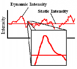
Across a long time interval, the dynamic signal appears to be representative of random fluctuations about a mean value. When viewed on a much smaller time scale however (inset in above figure), it is evident that the intensity trace is in fact not random, but rather composed of a series of continuous data points. This absence of discontinuity is a consequence of the physical confinement of the particles to be in a position very near to the position occupied a very short time earlier. In other words, on short time scales, the particles have had insufficient time to move very far from their initial positions, and as such, the intensity signals are similar. The net result is an intensity trace that is smooth, rather than discontinuous.
Correlation is a second order statistical technique for measuring the degree of non-randomness in an apparently random data set. When applied to a time dependent intensity trace, as measured with a dynamic light scattering instrument, the correlation coefficients are calculated as shown below, where t is the delay time.
![]()
Typically, the correlation coefficients are normalized, such that G(Ą) = 1. For monochromatic laser light, this normalization imposes an upper correlation limit of 2 for G(to) and a lower baseline limit of 1 for G(Ą). In practice, experimental upper limits for a DLS correlogram are typically around 1.8 to 1.9.
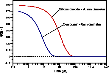
In dynamic light scattering instrumentation, a digital correlator continually adds and multiplies short time scale fluctuations in the measured scattering intensity, to generate the correlation curve for the sample. Examples of correlation curves measured for two sub-micron particles are given in Figure 2. For the smaller and hence faster diffusing protein, the measured correlation curve has decayed to baseline within 100 ms, while the larger and slower diffusing silicon dioxide particle requires nearly 1000 ms before correlation in the signal is lost.
In dynamic light scattering, all of the information regarding the motion or diffusion of the particles in the solution is embodied within the measured correlation curve. For monodisperse samples, consisting of a single particle size group, the correlation curve can be fit to a single exponential form as given in the following expression, where B is the baseline, A is the amplitude, and D is the diffusion coefficient. The scattering vector (q) is defined by the second expression, where ń is the solvent refractive index, lo is the vacuum wavelength of the laser, and q is the scattering angle.
![]()
![]()
The hydrodynamic radius is defined as the radius of a hard sphere that diffuses at the same rate as the particle under examination. The hydrodynamic radius is calculated using the particle diffusion coefficient and the Stokes-Einstein equation given below, where k is the Boltzmann constant, T is the temperature, and h is the dispersant viscosity.
![]()
A single exponential or Cumulant fit of the correlation curve is the fitting procedure recommended by the International Standards Organization (ISO). The hydrodynamic size extracted using this method is an intensity weighted average called the Z average.
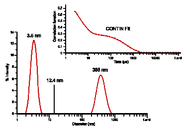
While the Cumulant algorithm and the Z average are useful for describing general solution characteristics, for multimodal solutions consisting of multiple particle size groups, the Z average can be misleading. For multimodal solutions, it is more appropriate to fit the correlation curve to a multiple exponential form, using common algorithms such as CONTIN or Non Negative Lease Squares (NNLS). Consider for example, the correlation curve shown in the figure below. This correlation curve, measured for a 10 mg/mL lysozyme sample in 100 mM NaCl at 69 C, clearly exhibits two exponential decays, one for the fast moving monomer at 3.5 nm and one for the slow moving aggregate at 388 nm. The size distribution was derived by fitting the measured correlogram to a multi-exponential using the CONTIN algorithm. When the single exponential Cumulant algorithm is used, a Z average of 12.4 nm is indicated. As evident here, the Z average, while beneficial for the purposes of citing a single average value, is clearly inadequate for giving a complete description of the distribution results.
The area under each peak in the DLS measured intensity particle size distribution is proportional to the relative scattering intensity of each particle family. The scattering intensity is proportional to the square of the molecular weight (or R6), and as such, the intensity distribution will tend to be skewed towards larger particle sizes. While this behavior is expected, it can lead to some confusion with new DLS users. Fortunately, a transformation of the intensity to a volume or mass distribution can be accomplished using Mie theory, wherein the optical properties of the analyte are used to normalize the effects of the R6 dependence of the scattering intensity. The assumptions required for the transformation are:
1) The particles can be modeled as spheres.
2) All particles have an equivalent and homogeneous density.
3) There is no error in the intensity particle size distribution.
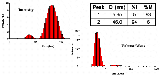
For many applications, the first 2 assumptions are reasonable. The third assumption however, will always fail, due to the ill-posed nature of the correlogram fitting in the DLS technique. In other words, regardless of how monodisperse the sample is, the DLS measured distribution will always have a small degree of inherent polydispersity, i.e. you’ll never be able to achieve a single band distribution as one might achieve using TEM measurements. As such, the volume transform should not be used to report particle size, but rather to report mass composition. Consider for example the figures shown below, which shows both the intensity and volume distributions for an ovalbumin sample in PBS buffer at 79 C. Two populations are evident – one at 6.0 nm and one at 46 nm. By intensity, the larger particle size family dominates the distribution, even though it represents only 6% of the total mass of the sample.
For additional questions or information regarding Malvern Instruments complete line of particle and materials characterization products, visit us at www.malvern.com.