How is the distribution calculated in DLS?

The particle size distribution from dynamic light scattering (DLS) is derived from a deconvolution of the measured intensity autocorrelation function of the sample. Generally, this deconvolution is accomplished using a non-negatively constrained least squares (NNLS) fitting algorithm, common examples being CONTIN, Regularization, and the General Purpose and Multiple Narrow Mode algorithms included the Zetasizer Nano software.

In photon correlation spectroscopy (PCS) or dynamic light scattering, single photons are detected and correlated. Correlation is a statistical method for measuring the degree of non-randomness in an apparently random data set. The autocorrelation function is the convolution of the intensity signal as a function of time with itself. When applied to a time dependent intensity trace, as measured in dynamic light scattering, the correlation coefficients, G(t), are calculated as shown below, where I is the intensity, t is the time, and t is the delay time.

The shift time (t) is often referred to as the delay time since it represents the delay between the ‘original’ and the ‘shifted’ signals. While the continuous intensity correlation function cannot be directly measured, it can be approximated with discrete points obtained by a summation over the duration of the experiment. The expression giving an approximation of the continuous autocorrelation function is shown below, which holds true for both linear and arbitrary delay times.

If the intensity statistics of the measured signal are Gaussian (which is true for all diffusion and for most random processes) then the Siegert relation holds true. The Siegert relation states that the normalized intensity autocorrelation function can be expressed as the sum of 1 and the square of the field autocorrelation function, g(t), scaled with a coherence factor g expressing the efficiency of the photon collection system.

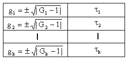
As with the intensity autocorrelation function, the Siegert expression can also be written in a discrete form with the index k. If we assume "ideal detection" where g = 1, then as a first approximation, a table of g_k and t_k values can be generated.

In the table above, the negative root value represents the unphysical case of G < 1, and is used to approximate the experimental noise within the real data. This approach imposes less bias than either restricting data to only the positive root or completely eliminating the G < 1 outliers.

The ideal field correlation function of ‘hypothetical’ identical diffusing spheres is given by a single exponential decay function with decay rate G determined by the diffusion coefficient and the wave vector of the scattered light. The main objective of the data inversion consists of finding the appropriate distribution of exponential decay functions which best describe the measured field correlation function. In mathematical circles this problem is known as a Fredholm equation of the first kind with an exponential kernel. It is also known as an ill-posed problem, since relatively small amounts of noise can significantly alter the solution of the integral equation.

The fitting function for g_k then consists of a summation of single exponential functions which is constructed as a grid of exponentials with decay rate G_i .

The factor A_i is the area under the curve for each exponential contribution, and represents the strength of that particular i^th exponential function. The best fit is found by minimizing the deviation of the fitting function from the measured data points, where a weighting factor s_k is incorporated to place more emphasis on the strongly correlated, rather than the low correlation (and noisy), data points.

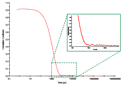
The weighting factor is proportional to the intensity correlation function value, i.e. correlation function values at small times have a higher weight than those at large times. Consider for example, the correlation curve shown in the figure below. As evident in the inset view, there is experimental noise in the baseline. In the absence of a weighting factor, this noise could be interpreted as ‘decays’ arising from the presence of very large particles.

Identifying the solution of A_i’s in the grid of fitted g_k expressions is accomplished by minimizing the deviation in x² with respect to each A_i, and then solving the resulting system of equations. If we construct the solution out of N exponential functions there will be N differentiations of the following form, where each of the differential terms contains a summation over all k.

The above system of equations can conveniently be re-expressed in matrix form as shown below, where the Y-vector turns out to be a convolution of the experimental data with the kernel (= the grid matrix or the exponential decays) and the matrix W consists of a convolution of the kernel with itself.

The standard procedure for solving the above equation is to find the eigenfunctions and eigenvalues, and then construct the solution as a linear combination of the eigenfunctions. When the eigenvalues are small however, a small amount of noise can make the solution extremely large. Hence the previous ill-posed problem classification. To overcome the problem, a stabilizer (a) is added to the system of equations. This parameter is called the regularizer, and with its incorporation, we are performing a first order regularization.

The above expression is called a first order regularization because the first derivative (in A_i) is added to the system of equations. The alpha (a) parameter or regularizer determines how much emphasis we put on this derivative. In other words, it defines the degree of smoothness in the solution. If a is small, it has little influence and the solution can be quite choppy; whereas a larger a will force the solution to be very smooth.

In addition to the smooth solution constraint, NNLS algorithms also required that the solution be physical; that is, all A_i be non-negative and uniformly constrained. In short, these additional constraints require that the summation of all A_i yields a finite number.

With the constraints discussed above, Z is minimized by requiring that the first derivatives with respect to A_i be zero. As indicated previously, this minimization corresponds to solving a system of linear equations in A_i. The solution of A_i values is found using an iterative approach called the gradient projection method.

A spherical particle with radius R_i will produce a correlation function with decay rate G_i according to the following expression, where D is the translational diffusion coefficient, q is the scattering vector, k_B is the Boltzmann constant, T is the absolute temperature, h is the viscosity, ñ is the solvent index of refraction, l is the laser wavelength, and q is the scattering angle.

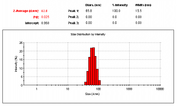
The normalized display of A_i vs. R_i (or A_i vs. diameter) is the intensity particle size distribution displayed within the Intensity PSD Report in the Zetasizer Nano software (see figure below). The average sizes displayed in the peak table are the intensity weighted averages, and are obtained directly from the size histogram using the following expression.

The peak width or standard deviation (s), indicative of the distribution in the peak, is also obtained directly from the histogram.

The figure below shows an excerpt from an Intensity PSD Report in the Zetasizer Nano software, and includes an example of the %Intensity histogram, along with the peak mean and standard deviation, derived from an NNLS deconvolution algorithm.

For additional questions or information regarding Malvern Instruments complete line of particle and materials characterization products, visit us at www.malvern.com.