In the dynamic light scattering (DLS) technique, the distribution of diffusion coefficients for a collection of particles is calculated by application of a multi-exponential fitting algorithm to the measured correlation curve. A common question from users of dynamic light scattering instrumentation is what is the best multi-modal algorithm.
One might initially feel that the question is ungrounded, in that the obvious best method for fitting the correlogram would be to use an iterative approach until the sum of squares error is minimized. For a perfect noise free correlation function, this approach would in fact be ideal. But in practice there is no such thing as a perfect noise free correlogram, and minimizing the sum of squares error in the presence of noise can lead to erroneous results, with no reproducibility and absolutely zero validity. So the question, "whats the best DLS algorithm", is a good question.
The problem with the whats the best algorithm question is that the answer is not a simple one, in that it depends very much on the type of samples being analyzed, the working size range of the instrument being used, and most importantly, the level of noise in the measured correlogram. There are a variety of "named" algorithms available to light scattering researchers, either through the web or through the collection of DLS instrument vendors. ALL of these algorithms are Non-Negative Least Squares (NNLS) based algorithms. What generally makes these named algorithms unique is the locking of variables (e.g. the "regularizer" or alpha parameter) within the NNLS algorithm, in order to optimize it for a given set of instrument and sample conditions. Some examples of named algorithms are:
CONTIN
The CONTIN algorithm was originally written by Steven Provencher and is has become the industry standard for general DLS analysis. CONTIN is considered to be a conservative algorithm, in that the choice of the alpha (a) parameter, which controls the "smoothness" of the resultant distribution, assumes a moderate level of noise in the measured correlogram. As a consequence, near in size particle distribution peaks tend to be blended together in a CONTIN derived size distribution. See http://s-provencher.com/pages/contin.shtml, for additional information.
Regularization
The Regularization algorithm, written by Maria Ivanova, is a more aggressive algorithm which has been optimized for dust free small particle samples, such as pure proteins and micelles. The Regularization algorithm utilizes a small a parameter, thereby assuming a low level of noise in the measured correlogram. As a consequence, Regularization derived distributions tend to have sharper peaks. However, this low noise estimate can also lead to phantom (nonexistent) peaks if noise is present in the correlogram.
GP & MNM
The GP and MNM algorithms, distributed with the Zetasizer Nano instrument, are general NNLS algorithms that have been optimized for the wide range of sample sizes and concentrations suitable for measurement with the Nano system. The GP (General Purpose) algorithm is conservative, with a moderate estimate of noise, and is suitable for milled or naturally occurring samples. The MNM (Multiple Narrow Mode) algorithm is more aggressive, with a lower noise estimate, and is better suited for mixtures of narrow polydispersity particles such as polystyrene latexes and pure proteins.
REPES & DYNALS
The REPES and DYNALS algorithms are available for purchase through various Internet sites. Both are similar to the industry standard CONTIN, although slightly more aggressive with regard to noise estimates.
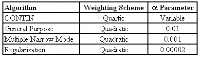
There are a variety of parameters that can be altered in an NNLS algorithm, the two principle ones being the "weighting scheme" and the "alpha parameter" or "regularizer". The table below shows a comparison of the default values of these two parameters for the major algorithms cited above. Note that the algorithms listed in the following table are listed in order of increasing "aggressiveness".
Data Weighting
Data weighting is used in DLS algorithms to amplify subtle changes in the larger and more significant correlation coefficients, over noise in the baseline. In the absence of data weighting, noise in the baseline can lead to the appearance of "ghost peaks" and erroneous data interpretation.
As an example of the merits of data weighting, consider the Zetasizer Nano measured correlation curve shown in Figure 1. This correlogram was derived from a 1 mg/mL Lysozyme sample, after filtration through a 20 nm Anotop filter. The inset in the figure shows a blow up of the baseline, and clearly indicates the presence of baseline noise.
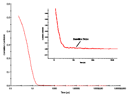
Figure 1: Zetasizer measured correlogram for a 1 mg/mL lysozyme sample, after filtration through a 20 nm Anotop filter.
The effect of the algorithm data weighting is to stretch out the correlogram along the Y axis (see Figure 2). This stretching acts to amplify subtle changes in the larger correlation coefficient values at smaller delay times, thereby decreasing the relative significance of noise in the baseline.
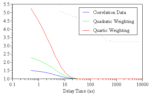
Figure 2: Comparison of quadratic and quartic weighting to the measured correlogram for a 1 mg/mL lysozyme sample, after filtration through a 20 nm Anotop filter.
A comparison of the intensity particle size distributions, derived with and without data weighting are shown in Figure 3, which indicates the presence of a particle family at circa 150 nm in the absence of data weighting. Since the sample was filtered prior to measurement, it is unlikely that the peak at circa 150 nm is real, but is more likely a "ghost peak" derived from noise in the baseline. When a weighting scheme is applied to the correlation data, the phantom peak is no longer present.
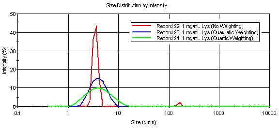
Figure 3: Comparison of intensity particle size distributions for a 1 mg/mL lysozyme sample, derived using the Malvern GP algorithm with and without data weighting.
Alpha (a) Parameter or Regularizer
The Regularizer or a parameter in NNLS based dynamic light scattering algorithms controls the acceptable degree of "spikiness" in the resultant distribution. Deconvolution of the DLS measured correlogram is accomplished using an inverse Laplace transform that is ultimately reduced to a linear combination of eigenfunctions. The caveat to this approach is that when the eigenvalues are small, a very small amount of noise can make the number of possible solutions extremely large. Hence the labeling of the method as an ill-posed problem. In order to overcome the problem, a stabilizing term, in the form of the "first derivative" of the distribution solution, is added to the set of eigenfunctions. The alpha parameter is the multiplier applied to this stabilizing term, and defines the emphasis placed upon the derivative of the solution. Large alpha values (0.1) limit the spikiness of the solution, leading to smooth distributions. Small alpha values (0.00001) decrease the weighting/importance of the derivative, subsequently generating more spiky distributions. The alpha parameter then, can be loosely described as an estimate of the expected level of noise in the measured correlogram.
There is no ideal or best alpha parameter. The appropriate value depends on the sample being analyzed. For mixtures of narrow mode (low polydispersity) and strongly scattering particles, decreasing the a parameter can sometimes enhance the resolution in the intensity particle size distribution. Consider for example, Figure 4, which shows the distribution dependence on the a parameter for a mixture of 60 and 220 nm latexes. The results derived using the default regularizer for the Malvern General Purpose and Multiple Narrow Mode algorithms, r = 0.01 and 0.001 respectively, are noted for comparison.
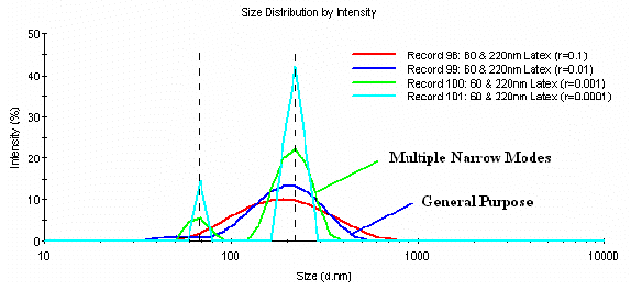
Figure 4: Intensity particle size distribution dependence on the a parameter for a mixture of 60 and 220 nm latex particles.
As evident in Figure 4, a decrease in the a parameter leads to an increase in both the number of resolved modes and the sharpness of the peaks. It is also important to note, that once baseline resolution is achieved, the resultant sizes (peak positions) are independent of the a value, with only the apparent width of the peaks changing with further changes in the regularizer. The relevance of this decrease in "apparent" peak width when the a value is decreased beyond that of the default value for the Malvern Multiple Narrow Mode algorithm is, again, dependent upon the type of sample. For the sample results shown in Figure 4, the sharper peaks are more representative of a bimodal mixture of latexes. If the sample is not composed of narrow mode particles however, aggressive reduction in the a parameter can quickly lead to over-interpretation of the measured data, and the generation of more modes/peaks than are actually present in the sample.
The influence of the a parameter on the measured size distribution for a monomodal 220 nm latex sample is shown in Figure 5. As with the mixture of latexes, reduction of the regularizer has no influence on the measured particle size, and serves only to decrease the apparent polydispersity of the peak, i.e. decrease the peak width. Since the Duke size standard measured here is known to be of low polydispersity, this sample would represent another example of where aggressive reduction of the a parameter generates a result that is consistent with the properties of the sample.
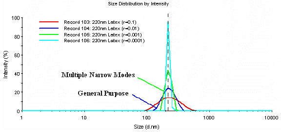
Figure 5: Intensity particle size distribution dependence on the a parameter for a monomodal 220 nm latex sample.
The influence of the a parameter on the resultant size distribution for a dilute protein sample is shown in Figure 6. Monomeric lysozyme has a known hydrodynamic diameter of 3.8 nm. Under the pH conditions employed here, lysozyme is also known to exist as mixture of low order oligomers, i.e. monomer, dimer, 4-mer, etc. As evident in Figure 6, the measured size of the sample is independent of the a parameter selected, and is consistent with an expected average size of a mix of lysozyme oligomers (> 6 nm). If the General Purpose algorithm is selected, with an a value of 0.01, the peak width is also representative of the expected polydispersity for a mix of protein oligomers. However, over-reduction of the a parameter (< 0.01) leads to the generation of a phantom peak at circa 2 nm. This phantom peak is a consequence of the reduced signal to noise ratio inherent to dilute protein measurements. As underestimate of the noise, by use of an aggressive a parameter, leads to the erroneous conclusion that the sample is composed of only two particle sizes, one of which is much smaller than the monomer itself. This sample then, is an example of a scenario where the larger a value generates results more consistent with the sample properties.
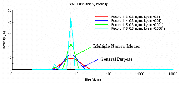
Figure 6: Influence of the a parameter on the resultant size distribution for a 0.3 mg/mL lysozyme sample in PBS at pH 6.8.
The results shown in Figure 7 represent another example where the less aggressive a value for the Malvern General Purpose algorithm is the appropriate one for use in the generation of the particle size distribution. In the absence of stabilizing agents, hemoglobin (Hb) denatures and aggregates at temperatures > 38 C. When the protein denatures, the aggregates formed are random in size, with no specificity, i.e. very polydisperse. As such, the distribution best representative of the actual sample is that generated using the Malvern General Purpose algorithm, with an a value of 0.01. Reduction of the a parameter to values < 0.01 leads to the generation of two apparently unique size classes in the 300 & 800 nm regions that are inconsistent with the actual properties of the sample.
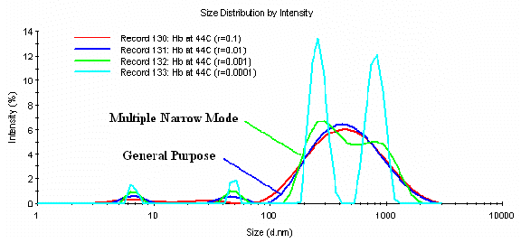
Figure 7: Influence of the a parameter on the resultant size distribution for denatured hemoglobin at 44 C in PBS buffer at pH 6.8.
With regard to the original premise of using an iterative fitting approach until the sum of squares error is minimized, Figure 8 shows the dependence of the sum of squares error on the a parameter for the four examples discussed above. The dashed lines in the figure represent the a parameter values for the General Purpose, Multiple Narrow Mode, and Regularization algorithms at a = 0.01, 0.001, and 0.00002 respectively. The circles indicate the a value identified in the above discussions as the most appropriate for the given sample. As seen in this figure, reducing the a parameter produces a better fit of the measured data and a subsequent reduction in the sum of squares error. However, selection of the "best fit" results is not always appropriate, especially if one is working with dilute and/or high polydispersity samples.
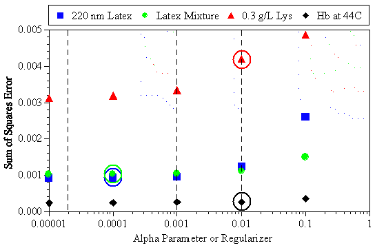
Figure 8: Dependence of the sum of squares error on the a parameter for the examples discussed above. The dashed lines represent the a parameter values for the General Purpose, Multiple Narrow Mode, and Regularization algorithms at a = 0.01, 0.001, and 0.00002 respectively. The circles indicate the a value identified as the most appropriate for the given sample
CONTIN
The CONTIN algorithm is unique among the commonly available DLS algorithms, in that it generates a collection of solutions, each with a set of qualifying descriptors that are used to select the most probable solution. The qualifying descriptors used to identify the most probable solution are 1) the number of peaks, 2) the degrees of freedom, 3) the a parameter, and 4) the probability to reject. The most probably solution is selected using the principle of parsimony, which states that after elimination of all solutions inconsistent with a priori information, the most appropriate solution is the one revealing the least amount of information that was not already known or expected.
Figure 9 shows a comparison of the CONTIN generated solution set for the 60 and 220 nm latex mixture discussed earlier. As seen in this figure, one of the solutions in the set (CONTIN 1) is consistent with the results generated using the Malvern Multiple Narrow Mode algorithm (a = 0.001) and is a good representation of the actual sample. However, the solution determined by CONTIN to be the most probable is the CONTIN 6, which shows a blending of the populations to form a single peak of high polydispersity.
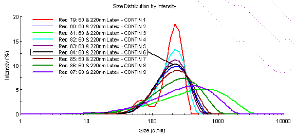
Figure 9: Comparison of the CONTIN generated solution set of size distributions for the DLS measured 60 and 220 nm latex mixture. Solution #6 is the most probable solution, as determined by CONTIN analysis.
In comparison to the Malvern General Purpose and Multiple Narrow Mode algorithms, CONTIN tends to be a little more conservative than the GP algorithm. While this works well for "noise" recognition and management (Dilute Protein in Figure 10), it can also lead to a reduction in apparent particle size resolution (Latex Mixture in Figure 10) for mixtures.
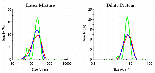
Figure 10: Comparison of CONTIN (ū), General Purpose (ū), and Multiple Narrow Mode (ū) results for a mixture of 60 and 220 nm latexes and a dilute protein (0.3 mg/mL lysozyme) sample.
In closing, to finally address the question of "what is the best DLS algorithm", the answer is that there is no best algorithm. All the algorithms give useful information to the researcher. The best approach is to couple what you know with what you suspect about the sample, compare results from various algorithms, recognizing the strengths and limitations of each, and then look for robustness and repeatability in the results. In other words, if multiple measurements all indicate a shoulder in a wide peak, which resolves itself into a unique repeatable population upon application of a more aggressive algorithm, the chances are strong that the this unique population is real. If repeat measurements generate inconsistencies, then it is best to err on the side of a more conservative algorithm, such as the Malvern General Purpose or CONTIN.
For additional questions or information regarding Malvern Instruments complete line of particle and materials characterization products, visit us at www.malvern.com.